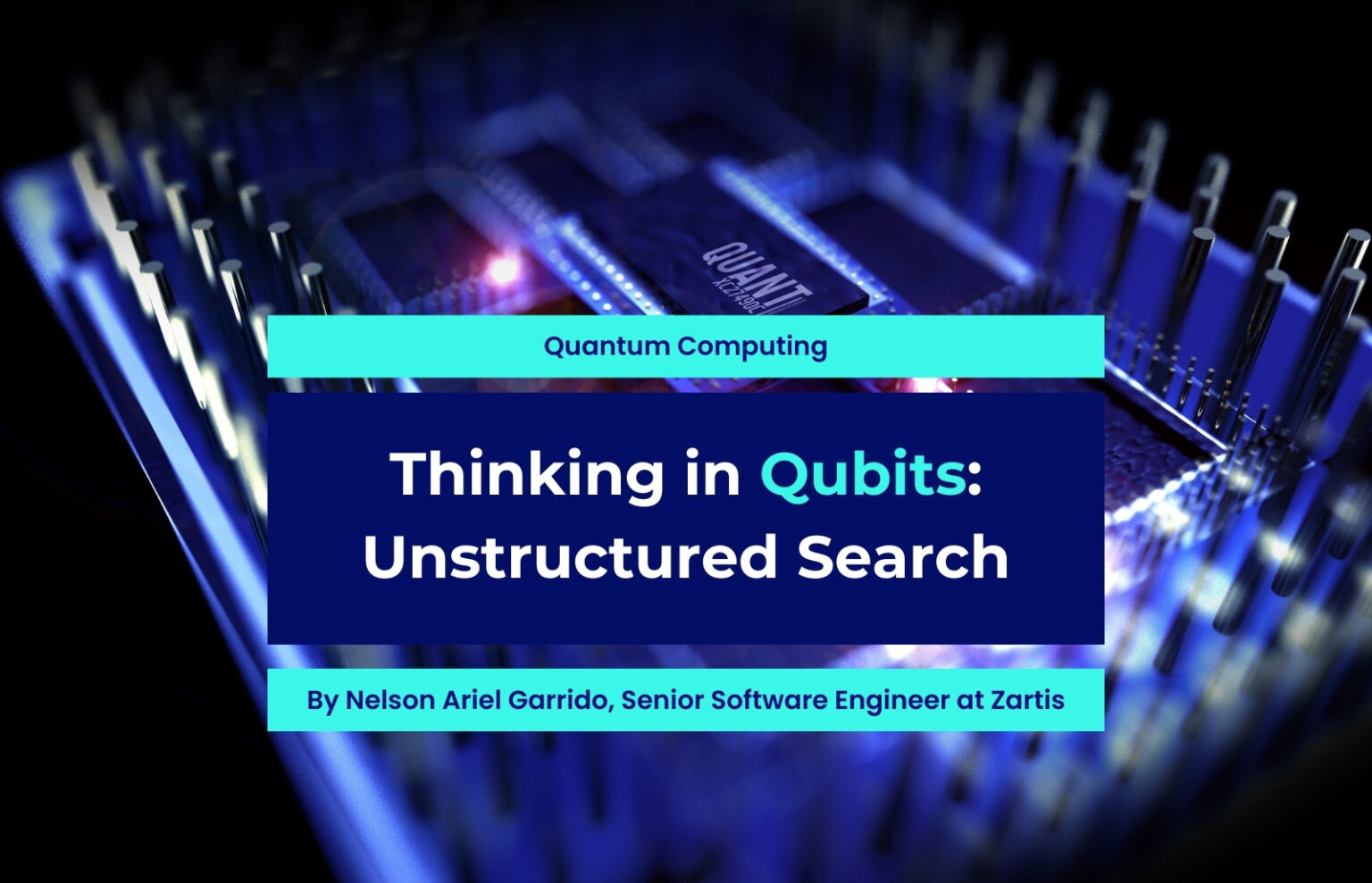
Imagine you have a large, unordered list of elements. For example, a telecommunications company manages a pool of valid SIM cards that are not organized in any specific way. When a customer request arrives, the company needs to verify whether a particular SIM card is included in that pool.
In a classical computing scenario, lacking any kind of ordering, this problem can only be solved through a sequential search—that is, by examining each element one by one until the desired one is found. The most efficient algorithm in this case is linear search, with a computational cost of O(N) in the worst case, where N is the total number of elements. Statistically, if the element is randomly distributed, the average number of steps required is N⁄2. This means that if there are one million SIM cards, on average, about 500,000 would need to be checked before finding the right one.
But what if we had access to a quantum computer? In that case, we could use Grover’s algorithm, one of the most well-known quantum computing solutions for searching in unsorted and unstructured databases. It can locate the target element with a quadratic speedup over the best classical algorithm, reducing the number of required steps from N to approximately √N. This improvement becomes especially relevant in large-scale problems, where search time can be a critical factor.
How Does Grover’s Algorithm Perform a Search?
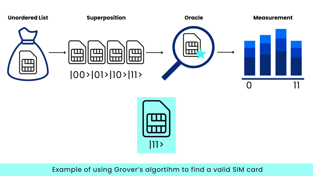
Grover’s algorithm is based on a sequence of quantum transformations applied to a set of qubits using logic gates. Its conceptual structure is shown in Figure 1, where three main phases can be distinguished:
- Preparation of a uniform superposition of all possible states.
- Application of an oracle that modifies the phase of the marked state.
- Amplitude amplification through a diffuser (reflection about the mean).
To facilitate its analysis and implementation, this work focuses on a 2-qubit system, which generates a search space of four possible states. This choice is intended to simplify the implementation and make the algorithm’s dynamics easier to observe, while also aligning with the current limitations of quantum computing hardware, where both the number of available qubits and the fidelity of quantum gates remain restricted.
For the practical implementation, the IBM Quantum Composer tool is used—a visual platform that allows users to design and simulate quantum circuits step by step using basic logic gates.
As an illustrative case, the algorithm is implemented to search for the marked state ∣11⟩, that is, the last of the four possible states in a 2-qubit system. This choice is not arbitrary: in the context of the introductory example—the search for a specific SIM card within an unordered database—the state ∣11⟩ can represent the presence of a valid SIM at the final position of the list. The algorithm enables us to locate this state without sequentially examining all the elements, thus demonstrating its quantum advantage. The implementation shows how the probability of that state is gradually amplified until it becomes the most likely result upon measurement.
1. Preparation of a Uniform Superposition
In classical computing, a bit can only exist in state 0 or 1. In contrast, a qubit can exist in a superposition of both states. This property is achieved through the Hadamard gate (H), which transforms the base state ∣0⟩ into a balanced combination:
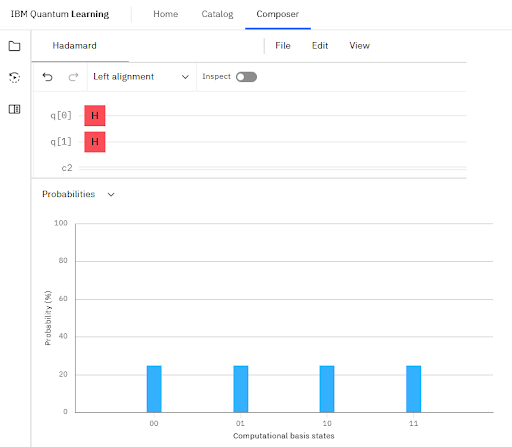
By applying Hadamard gates to all the qubits in the system, a uniform superposition of all possible states is created. For example, with 2 qubits, 4 combinations are generated, each with the same amplitude. Figure 2 shows how this superposition operation is implemented in IBM Composer.
2. Oracle Application
The oracle is a fundamental subroutine. Its role is to mark the target state by modifying its phase: it applies a multiplication by −1 to the amplitude of the desired state. This transformation does not directly alter the probability of measuring that state, but it introduces a key difference at the quantum level.
At this point, we might ask: what is *phase*? It is a property unique to qubits—something that classical bits do not possess. One can imagine it as the angle at which an arrow rotates around the Bloch sphere, the geometric space used to represent a qubit’s state. While a classical bit can only take the values 0 or 1, a qubit can exist in a superposition of both, and also have a direction of rotation that defines its relative phase. Although this phase does not directly affect the measurement outcome of a qubit, it does influence how quantum states interfere with one another—an essential feature for the operation of this algorithm.
This transformation does not directly change the measurement probability of that state, but it introduces a crucial distinction: it allows the next stage (the diffuser) to turn this phase modification into an effective advantage.
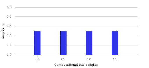
Since we are working with 2 qubits, the state space contains 4 possible combinations. Figure 3 shows the visualization prior to applying the oracle, where all amplitudes are equal and phases are positive.
After applying the oracle, the phase of the target state is inverted. In Figure 4, this inversion is represented by a color change. Although invisible to direct measurement, this “quantum mark” is essential for the next stage.
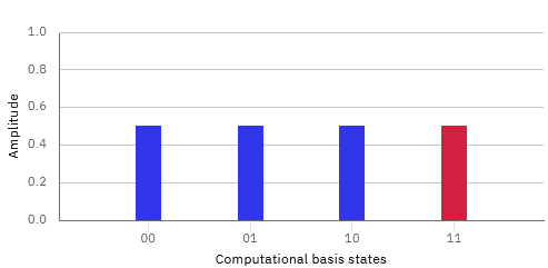
This mechanism, though simple, is extremely powerful: it allows the algorithm to “recognize” the correct state without explicitly checking all possibilities. In this sense, the oracle acts as a hidden mark that guides the quantum computing process toward the solution.
3. Amplitude Amplification (Diffuser)
After marking the desired state, the next step is to amplify its probability (Figure 5). This is done using the diffuser, which operates by reflecting the amplitudes with respect to the global average.
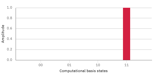
The diffuser reflects the amplitudes of all states around the global mean. Since the amplitude of the marked state was inverted by the oracle, it lies below the average. When the diffuser is applied, this amplitude increases, while those of the other states are slightly reduced. Repeating this process several times concentrates the probability on the correct state—not by explicitly eliminating others, but through constructive and destructive interference.
4. Measurement
Finally, after an appropriate number of iterations (approximately √N, where n is the number of qubits), the system is measured. At this point, the probability of collapsing into the marked state is the highest.
It is important to note that measurement causes the quantum state to collapse into a classical state. However, thanks to the amplification process, this collapse occurs with high probability on the correct state, thus solving the search problem with quantum efficiency.
Implementation of Grover’s Algorithm in IBM Quantum Composer
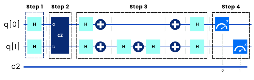
Figure 6 shows the practical implementation of Grover’s algorithm using IBM Quantum Composer, a visual platform that allows users to design, simulate, and analyze quantum circuits step by step. In this case, as previously discussed, a circuit is built to identify the marked state ∣11⟩ within a 2-qubit system, which corresponds to an unordered database of 4 elements.
Step 1: Superposition Preparation
Hadamard (H) gates are applied to both qubits. This operation transforms the base state ∣00⟩ into a uniform superposition of the four possible states (∣00⟩, ∣01⟩, ∣10⟩, ∣11⟩), each with equal amplitude. This initial superposition serves as the starting point of the algorithm, allowing all states to be considered simultaneously.
Step 2: Oracle Application
To mark the ∣11⟩ state, a controlled-Z (CZ) gate is used to invert its phase. In quantum circuits, this phase inversion is represented as a multiplication by −1 of the corresponding amplitude, without affecting its measurement probability. If the target state were different (e.g., ∣10⟩), X gates would need to be applied before and after the CZ gate to change the control basis and correctly mark the desired state.
This step serves to “label” the correct state through a quantum mark that is invisible to direct measurement but essential for the constructive interference that occurs in the next stage.
Step 3: Diffuser (Amplitude Amplification)
Once the target state is marked, the diffuser is applied, also known as an inversion about the mean. In IBM Composer, this is implemented with the sequence: H → X → CZ → X → H
This pattern reflects the amplitudes of all states with respect to the global meaning. Since the ∣11⟩ state now has a negative amplitude (due to the oracle), it lies below the average. The reflection projects it above the mean, increasing its probability. In larger systems, this cycle (oracle + diffuser) must be repeated multiple times, but with 2 qubits, a single iteration is enough to observe the amplification effect.
Step 4: Measurement
Finally, both qubits are measured. Since the probability of the ∣11⟩ state has been amplified, it becomes the most likely outcome after measurement, thereby validating the algorithm’s efficiency compared to classical search.
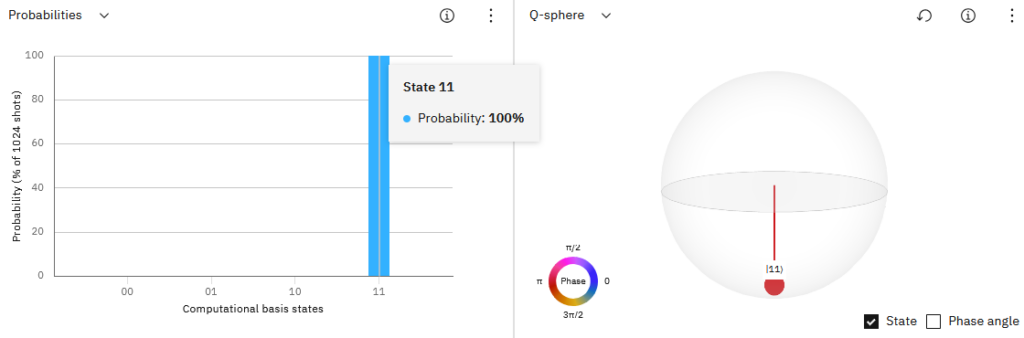
IBM Quantum Composer allows for complete circuit simulation and result visualization (Figure 7) in two key formats:
- Measurement histogram: hows that the ∣11⟩ state has a significantly higher probability than the others, as a result of the amplification process.
- Statevector and Bloch sphere: allow for the observation of not only amplitude distribution but also the relative phase of each state property unique to quantum systems.
This practical implementation clearly illustrates how a small number of quantum gates can solve an unstructured search problem with an advantage over classical methods. Moreover, it serves as a foundation for future extensions of the algorithm to larger search spaces or more complex problems.
Conclusion
Beyond the theory, the simulation in IBM Quantum Composer demonstrated how this quantum computing process is built and executed step by step: from preparing the system in superposition, to applying the oracle and the diffuser, and finally measuring the target state. The result is not just a working circuit, but a concrete entry point into the potential of applied quantum computing algorithms.
However, it is important to acknowledge that the current state of quantum computing still presents significant limitations: the number of available qubits, gate fidelity, and the presence of noise mean that, for now, only reduced versions of these algorithms can be feasibly implemented. Even so, exercises like this allow us to explore the foundations of a technology that promises, over time, to transform the way we solve complex problems.
—
If you’d like to connect with our team of experts and learn more about this topic, please feel free to reach out!
Author: